Meshless Mania

Simulation Democratisation Series Part 1

Written by Nirav Mota, Team Lead - Durability Simulation at Ather Energy

INTRODUCTION

In the fast-paced engineering sector, simulations are essential for virtually testing designs, predicting outcomes, and optimising performance. The Finite Element Method (FEM) has been the gold standard in structural analysis for many years; however, the emergence of meshless simulations is ushering in a new era of democratisation, allowing designers to accelerate the speed of engineering execution. Ather Energy, known for using simulations to develop best-in-class reliable products, has seen significant gains in speed and innovation using meshless simulations. This article provides a brief overview of these advancements & dives into fundamental math of methods involved.

Why Meshless?

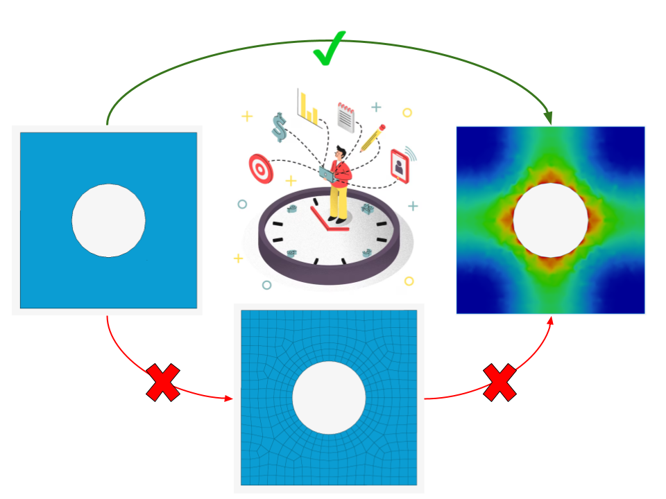
A reasonable question is "why explore meshless simulations as we already have the FEM that solves engineering problems?". The simplest answer is that a modeling with Finite element analysis (FEA), while generally accurate and repeatable for many engineering problems, can be ineffective and laborious for certain types of simulations. A potential alternative, meshless simulation (also known as mesh-free simulation) eliminates the traditional mesh structure used in FEA. Rather than dividing the simulation domain into small elements, meshless simulations represent the geometry with a distribution of points. This makes them more flexible and easier to set up than traditional FEA.

Meshless simulations are ideal for engineering applications that require rapid prototyping and quick iteration, as they can easily handle complex geometries and large deformations.

Math of Meshless

In Ather’s context, understanding physics, narrating it with first principles and solving it with math & tools, makes an engineer we cheer for. It is very critical to understand how meshless solvers work even if we were to apply it in engineering practice to reap the fruits.

To understand the difference between FEM and Meshfree solver workflows, let's take a classic (& my personal favourite) engineering challenge ’a cantilever beam subjected to a point load at its free end’ example. We'll examine the steps involved in finding the displacement and stress solutions using each method.

Problem Statement:

Consider a cantilever beam with the following specifications:

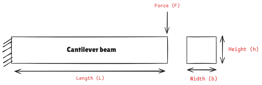
Length L = 100 mm , Width b = 10 mm, Height h = 10 mm, Young's Modulus E = 210,000 MPa

Moment of Inertia I = 833.3333 mm⁴

Applied force at the tip of free end F = 600 N

Maximum bending moment M = F L = 60000 Nmm

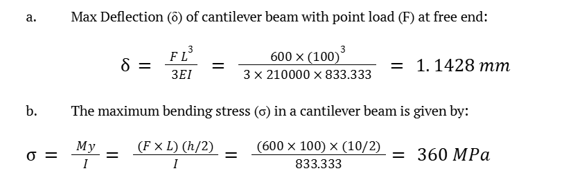
Now, with the analytical solution available, let’s understand the FEM and Meshless method (Element-Free Galerkin - EFG) solution procedure for the same cantilever beam.

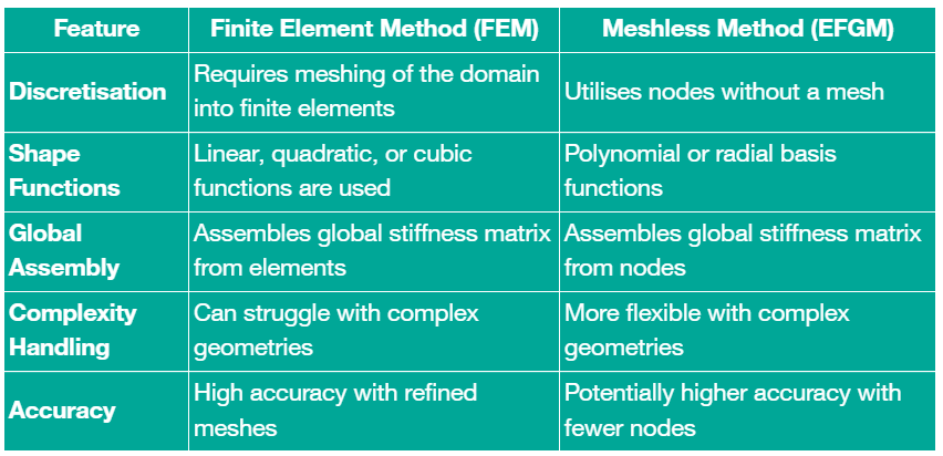
Let's start with the basic difference between FEM and Meshless solver workflow.

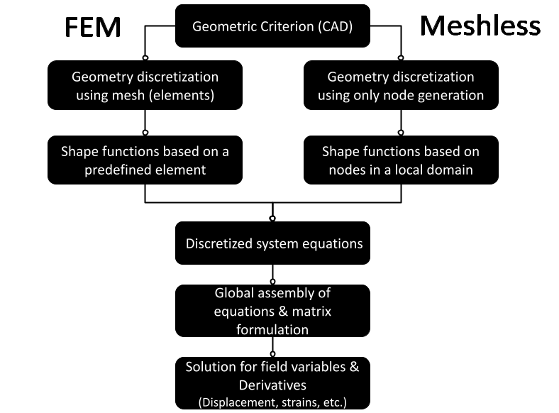
1. Geometry discretisation

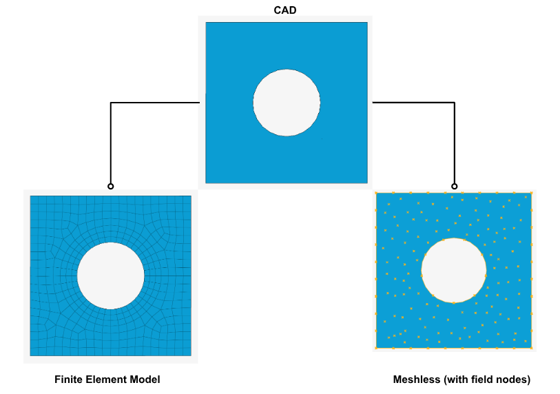
It's a very common misconception that meshless techniques don't require discretisation. The workflow above shows that meshless techniques are faster because they don't need mesh generation and can solve problems with node generation alone to represent the geometry.

In meshless methods, nodes are scattered across the problem domain and its boundary. These nodes, often called field nodes, carry the values of the field variables. Node density depends on the required accuracy and available resources, and the distribution is usually non-uniform. Adaptive algorithms can control node density automatically, making the initial distribution less important. This significantly reduces the reliance on skilled labor for generating finite elements with a reliable quality matrix to capture the geometry, which is a major challenge in the preprocessing stage. The image below provides a quick reference for discretisation.

a. FEM:

For our cantilever beam, we might choose to divide it into n linear equal length (L_e) beam elements. Each element has nodes at its ends, and the beam can be represented as follows:

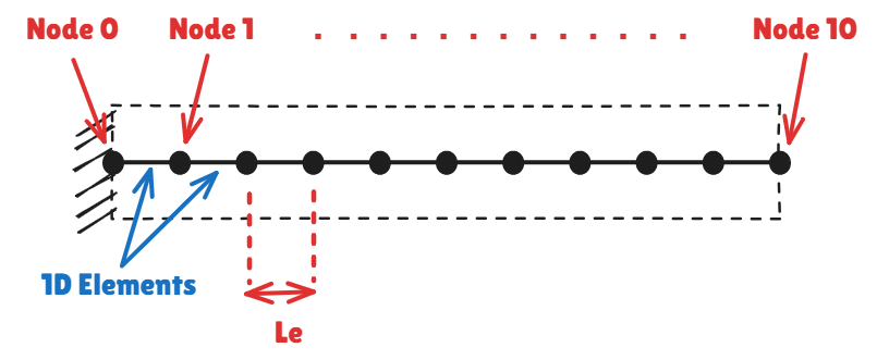
*This explanation uses 1D Beam elements to model the FEM, for the sake of simplicity, rather than 2D or 3D meshed models. The same approach applies to 2D & 3D FEM models, but the matrix formulation & solution is more complex (and beyond the scope of this article).

Element properties are then determined by global inputs and the number of nodes/elements. For example, length of each element:

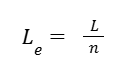
Similarly, the Young’s modulus, cross-sectional area, Poisson’s ratio, and related parameters are defined for each element in accordance with user specifications.

b. Meshless:

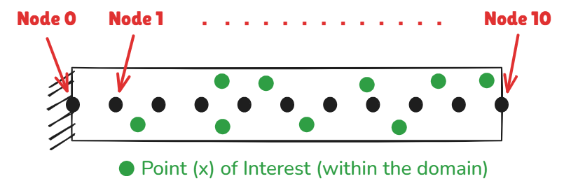
In the meshfree (Element-Free Galerkin used for this article) method, we start by defining a set of nodes along the length of the cantilever beam. For simplicity, let's place nodes at equal intervals.

Let's use 11 equally spaced nodes along the beam length:

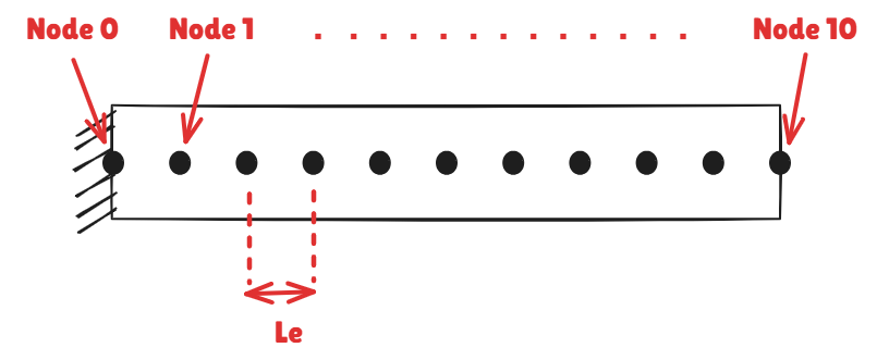
Thus, to interpolate the nodal co-ordinates of these individual nodes,

x_i = i . L_e

Where, L_e = Distance used for creating equidistance nodes for our beam

i = Node number

The node coordinates will be:

Node 0: x₀ = 0 mm (fixed end)

Node 1: x₁= 10mm

Node 2: x₂ = 20mm

…

Node 10: x₁₀ =100mm (free end)

2. Local Formulations

This step deals with elemental / node level formulations to build up models which then can be solved using mathematical approaches.

a. FEM:

For a 1D beam element, the elemental stiffness matrix K_e is given by:

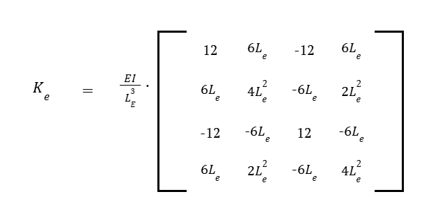
Substituting the appropriate values yields the local stiffness matrix for each element.

b. Meshless:

In absence of elements, shape functions are defined for each node. Polynomial functions or radial basis functions are commonly used shape functions. In this instance, we will use a simple polynomial shape function:

For a linear shape function associated with node i :

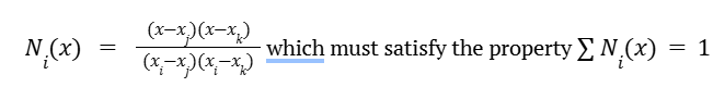
Where j and k are neighboring nodes. x is any point within the problem domain interpolated using function values at field nodes (initial nodes created using discretisation).

Next, these shape functions are leveraged to derive a weak form solution such that it can be used for global matrix formulation in the further steps.

The beam's behavior is derived from the weak form of the governing equations. The governing equation for the bending of beams is given by

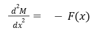
Where M is the bending moment and F(x) is the applied force. The weak form involves multiplying by a test function v(x) and integrating over the domain:

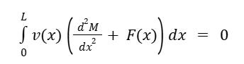
This method basically turns a differential equation into an integral one, which is usually easier to solve on a computer. It says the weighted error has to be zero, no matter what test function v(x) you use. The cool thing is we can use simple, piecewise polynomial approximations (those shape functions) instead of needing a really complicated, always-correct equation.

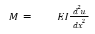
The bending Moment M can be expressed using Euler’s equation relating it to filed displacement u

And for given point x, the displacement u(x) can further be represented by weighted sum of shape functions:

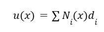
Here, d_i is the nodal displacement at i^th node.

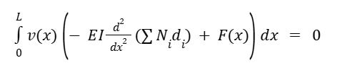
Substituting these into the weakform equation we get

3. Assembly of locals to formulate global matrices

a. FEM:

Assemble the global stiffness matrix K by summing up individual element stiffness matrices, ensuring correct mapping of degrees of freedom (DOF) across elements.

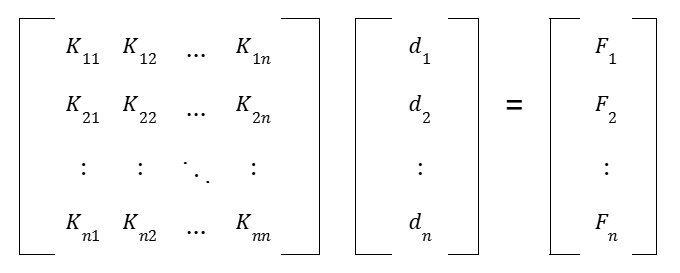
Where, d_i are the nodal displacements and F_i are the nodal forces.

The global stiffness matrix K is assembled based on the contributions from each element. The resulting system of equations is:

K { d } = { F }

Where,

{ d } is the vector of unknown nodal displacements.

{ F } is the global force vector.

b. Meshless:

The weak form derived in the previous step now involves integrals that can be computed based on the shape functions and nodal displacements. Each node contributes to the overall stiffness matrix and force vector according to its local shape functions. Specifically, we can compute the contribution of each node to the global system by evaluating the integrals:

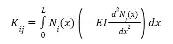
This integral represents the contribution of the j^th node's shape function to the stiffness associated with the ith node.

Assemble the global system of equations from the contributions of all nodes. Each term contributes to the global stiffness matrix K and force vector F:

K { d } = { F }

Where,

K is the global stiffness matrix assembled from local contributions.

{ d } is the vector of unknown nodal displacements.

{ F } is the global force vector.

4. Solve for the unknowns (field variables like displacement)

a. FEM:

By applying boundary conditions to the global system, we can take the first step towards a solution. In the case of a cantilever beam, the node at the fixed end has zero displacement and rotation. As a result of this step, the number of unknowns in a single row of matrix equations is reduced, making it solvable.

Further, to solve for the unknown variable, nodal displacement { d_i } at respective nodes, use matrix operations to solve for each row (Easier said than done using hand calculations and hence, I am ever thankful to Charles Babbage!).

b. Meshless:

Similar to FEM, boundary conditions must be applied to the meshless formulation. For our cantilever beam, the displacement at the fixed end (node 0) is set to zero.

Once the global system of equations is solved for the unknown nodal displacements { d_i } at respective nodes, the deflection at the free end can be computed using the nodal values derived from the shape functions.

5. Post processing (“Picture abhi baaki hai mere dost!”)

Phew! Finally we have our first unknown “Displacement”. But what about the STRESS or other outputs that we end up looking to gain more insights on durability (or to make the report more colourful!)?

One might be quick to suggest that since we have displacement, we can calculate the strains and then, using Hooke's law, determine the stress values, hurrayyyy!! While this works for most of cases analytically (most of because of a twister called non-linearity), FEM or Meshless method rather relies on a more engineered version of arriving at this.

For example, consider this. Strain (and resulting stress) isn’t really a nodal value. For strain to appear, something with “initial length” must change its length. Do Nodes have length at all…?

This is where unsung heroes named “Shape Functions” are called for. Shape functions are essential for interpolating the solution within an element / local domain based on nodal values. It can be linear polynomial, or of higher order (quadratic, cubic) depending on the complexity of the physics and accuracy sought for. However, math for getting into generating and solving it, we will park for another day.

In summary, both FEM and Meshless solvers utilise nodal results (starting with displacement) to obtain post-processing results (like strain and stress) using shape functions. The key distinction lies in the shape functions: FEM employs predetermined element shapes for easier creation of shape functions (and repeatability), while Meshless solvers generate polynomial or radial basis functions based on the desired solution complexity. This Meshless approach adapts to the number of nodes used for geometry discretisation, offering flexibility.

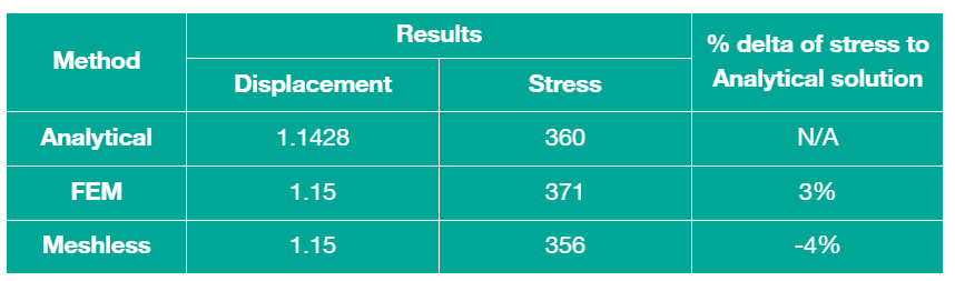
Time for results

Let’s look at results from actual professional tools using the FEM and Meshless methods to look at results in-comparison of analytical solutions for our beloved cantilever beam.

a. FEM

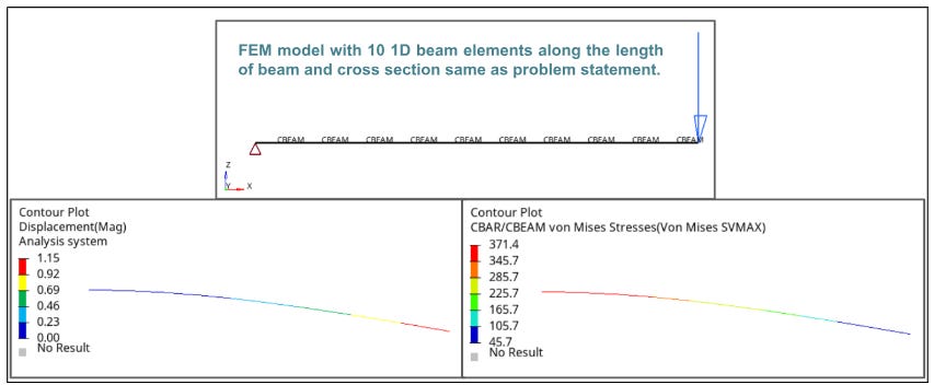
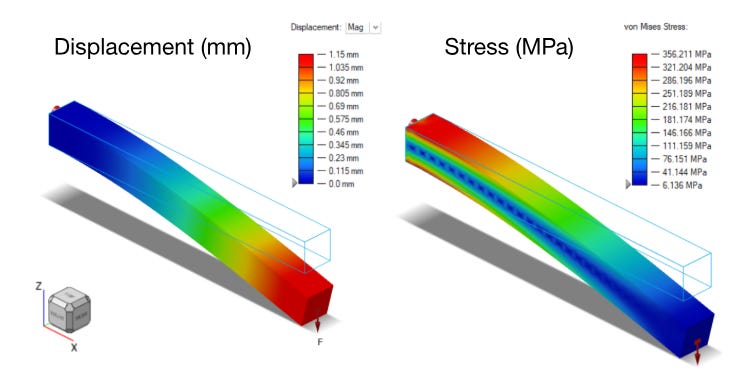
b. Meshless:

The results from using a meshless method tool are quite similar after a few adjustments to the adaptive settings. These settings can vary depending on the application, so it's best to use your engineering judgment initially.

Summary of Method Comparison

And here’s the result summary telling me that meshless is as good!

Conclusive Remarks

I still remember my engineering days where I could not get enough of FEA, never missing an opportunity to utilise the same for complex (at least I thought!) engineering projects. Comes the time in the corporate world & things need to be engineered at rocket pace. It’s all about the competitive markets driving the cycles and no one wants to be left behind. In such times, why not leverage the tech & collective mindset to drive the innovative cycles to deliver the best with record times. Meshless is just the start of it (on the tech front obviously); within the Ather, we foresee AI & Geometric deep learning helping us drive the virtual validations with the ‘firsts of its kind’ in the (EV) industry! Stay tuned for the developments.

References:

1. An Introduction to Meshfree Methods and Their Programming by G.R. LIU National University of Singapore, Singapore and Y.T. GU National University of Singapore, Singapore

2. Łukasz Skotny Ph.D , Can You do Finite Element Analysis by Hand?, 2019

3. WT Ang, A Beginner’s Course in Boundary Element Methods, Universal Publishers, Boca Raton, USA, 2007

4. USING ALTAIR SIMSOLID™ TECHNOLOGY OVERVIEW by Victor Apanovitch – SimSolid Senior Vice President, Altair